AI, Biological Data, and the Messy Reality of Biology

Jan 11, 2026

Introduction

Artificial intelligence (AI) and machine learning (ML) have revolutionized data analysis in biology, from genomics to medical imaging. These algorithms, however, often assume that the input data is clean, complete, and representative of the true biological signal. In theory, if we feed an ML model well-curated, noise-free data that perfectly captures the biology of interest, the model can learn meaningful patterns. In practice, real biological datasets violate these assumptions. Experimental data are frequently incomplete, noisy, and context-dependent, meaning that what an AI learns may reflect technical artifacts or sampling biases rather than true biology. This gap between assumption and reality is a central theme in modern bioinformatics and biomedical data science[1][2].

Why does this matter? When an AI model is trained on flawed or biased data, its predictions can mislead scientists or clinicians, leading to irreproducible results or even harmful decisions. For example, a model might latch onto laboratory-specific quirks (batch effects) or hospital-specific image features instead of genuine disease markers. As we will explore, recent research across genomics, transcriptomics, and medical imaging has revealed how data issues — missing values, batch effects, measurement error, loss of context — undermine AI models if not properly addressed.

In this manuscript, we present a two-level discussion of this principle. First, we provide a high-level, conceptual overview accessible to upper-level undergraduates, using intuitive analogies and simplified examples to illustrate why “messy” data confound AI. Next, we delve into a technical discussion of specific challenges in biological datasets (missingness, noise, batch effects, context dependence) and review open-access studies that demonstrate these problems in real-world applications. Throughout, we emphasize themes of reproducibility, careful data interpretation, and model robustness (or brittleness) in the face of data imperfections. We also highlight case studies and link to openly available datasets that have been instrumental in revealing these issues.

Our goal is for students to grasp conceptually why biological data often break the ideal assumptions of AI, and for instructors and advanced readers to gain a deeper technical understanding — and confidence — to navigate these challenges in practice. By the end, readers should appreciate not only the pitfalls that can arise when applying AI to biological data, but also best practices to improve reproducibility and reliability in their own data science endeavors.

Conceptual Overview: Why “Messy” Data Confound AI

AI algorithms are like very picky students: they learn best from examples that are clear and consistent. Classic ML theory typically assumes that data are independent and identically distributed (i.i.d.), fully observed (no missing parts), correctly labeled, and primarily differ due to the underlying phenomena of interest — not due to random noise or irrelevant factors. In simple terms, AI expects a clean photo album of biology. However, biological reality is more like a scrapbook – pages torn out, coffee stains on some images, and pictures from different events all mixed together. Below, we introduce in simple terms the key ways biological data deviate from the AI ideal:

· Incomplete Data (Missingness): Biological datasets often have missing values or unmeasured features. For instance, a patient’s medical record might lack some lab tests, or a multi-omics study might not measure every molecule in every sample due to cost or sample quality[1]. Standard AI models assume every feature is present for every example; missing data violate this assumption.

· Noise and Measurement Error: Laboratory measurements and clinical observations come with random errors and variability. Two labs measuring the same gene expression might get slightly different numbers; an X-ray image might be blurry or a clinician’s diagnosis might be subjective. These errors and noise can obscure true patterns. AI models assume the data reflect true signal, not a mix of signal + noise[3][4].

· Batch Effects (Technical Variability): Data collected in different batches – say, on different days, by different technicians, or with different equipment – can show systematic differences unrelated to biology[5]. It’s as if each batch has a hidden “fingerprint”. AI may mistakenly learn these fingerprints instead of the biology, unless we correct for them.

· Loss of Context / Context Dependence: Biological data are highly contextual – the conditions of an experiment, the population studied, or the environment can drastically change what the data mean. When context isn’t fully captured or changes between training and deployment, models can become biased or brittle. For example, a model trained on one hospital’s images may fail at another hospital because of different machine settings or patient demographics[6][7]. The model assumed the training context was universal, which often isn’t true.

Analogy: Imagine teaching a student to distinguish cats vs. dogs using only clear, close-up photos of pets taken indoors. The student (or AI) might learn to rely on subtle cues like fur patterns. But if you then show a blurry outdoor photo or an image missing half the animal, the student will struggle. Worse, if all indoor photos happened to be of cats and outdoor photos of dogs, the student might simply learn “indoors = cat, outdoors = dog.” In this analogy, the blurry or partial photos represent noisy and missing data, and the indoor/outdoor correlation is like a batch/context effect. The student’s “cat detector” would actually be detecting background differences — a spurious pattern.

In real biological problems, such confounders abound. AI models, being powerful pattern finders, will exploit any consistent signal to improve training accuracy – even if that signal is an artifact. This leads to models that perform well on the specific dataset (where the artifacts are consistent) but fail in genuine settings, or that yield biologically misleading conclusions. In the next sections, we examine each of these challenges in depth, citing recent research that exposes the consequences of assuming data are clean when they are not.

Challenges of Biological Data for Machine Learning (Technical Discussion)

Missing and Incomplete Data

One fundamental challenge in biology is missing data. Unlike a neatly organized spreadsheet, biological datasets often have holes: patients skip appointments (missing clinical data), sequencing machines fail to read certain genes, or multi-omics studies lack one of the omics for some samples. Missingness can be non-random, meaning the fact that data are missing might itself relate to the biology or study design (e.g., expensive assays done only on a subset of samples, or sicker patients more likely to have incomplete records).

Many AI/ML methods do not handle missing values natively – they either require imputation (filling in gaps) or they drop incomplete samples, which can introduce bias[8]. Crucially, if entire subsets of data are missing systematically, the model’s training data cease to be representative of reality. For example, in electronic health records, patients with lower socioeconomic status often have spottier data (less frequent visits, fewer recorded labs); a model trained on the observed data may underperform or give biased predictions for these groups[9][10]. Gianfrancesco et al. note that missing data in EHRs is a major source of bias and can affect which patients an algorithm identifies or ignores[9]. In other words, who or what is missing in the data can skew an AI’s perspective on the population.

In cutting-edge fields like multi-omics, missing data is practically the norm. A recent review by Flores et al. (2023) highlights that when integrating multiple ’omics (e.g., genomics, transcriptomics, proteomics) on the same specimens, “all biomolecules are not measured in all samples” – due to cost or technical issues – and many integration techniques assume access to completely observed data[1]. Methods that blindly assume every sample has every type of data will break. In response, researchers are developing specialized algorithms to handle partial data, ranging from statistical methods to AI-driven imputation[11]. For instance, some approaches pre-train on large public databases (like The Cancer Genome Atlas (TCGA), an open repository of multi-omics cancer data) to learn cross-omic correlations, then fill in missing measurements in a smaller target dataset[12][13]. One study showed that a deep learning model’s performance “diminished with increased missingness” in the data[14], underscoring quantitatively that the more data are missing, the worse typical models perform. This performance drop makes intuitive sense — it’s like trying to recognize a face with pieces of the photograph torn away.

Open data example: The TCGA program (The Cancer Genome Atlas) provides multi-omics datasets for thousands of tumor samples (including genomic DNA, RNA expression, methylation, etc.), openly available to researchers. However, not every tumor in TCGA has every data type; some might have DNA and RNA data but missing proteomics, for example. Any AI model built on TCGA must account for these gaps. Indeed, integrating TCGA data required methods like ComBat-Seq or matrix factorization to handle technical and missing-data issues[15][16]. Another resource, the Gene Expression Omnibus (GEO), hosts thousands of open gene expression datasets from different studies. If one attempts to combine multiple GEO datasets for a meta-analysis, they will encounter missing values (genes not measured in one study vs another) and must use imputation or intersection of features to make the data align. These open resources have been invaluable for developing and testing missing-data handling methods.

In summary, incomplete data can lead to incomplete or biased models. An AI trained on perfect records may crumble when faced with real-world data full of holes. Awareness of missingness has grown, and modern workflows stress transparency about missing data, using imputation carefully, and designing models (like certain Bayesian approaches or tree-based models) that can tolerate missing inputs. The key is to recognize that missing data aren’t just an inconvenience — they can fundamentally alter what patterns an AI learns if not dealt with, as documented in numerous biomedical ML studies[17].

Batch Effects and Technical Variability

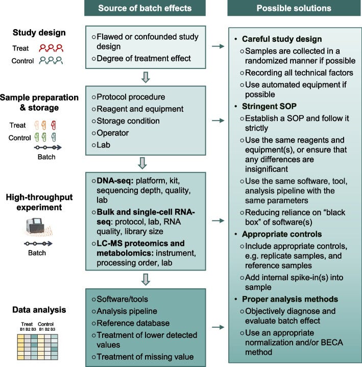
Fig. 1: Illustration of batch effects – unwanted technical differences between data subsets – and strategies to mitigate them. Sources of batch effects occur at all stages: study design (e.g. non-random sampling), sample handling (different protocols, storage), data generation (different machines or reagent batches), and analysis (different pipelines)[18][19]. These hidden influences can shift or distort measurements, requiring post-hoc correction or careful experimental design. The figure outlines common batch effect sources (left) and potential solutions (right), emphasizing that addressing batch effects is crucial for reliable, reproducible results[20]. For example, using randomized study designs, standardizing protocols, and applying computational batch correction (like ComBat or mutual nearest neighbors for single-cell data) can help align data distributions across batches.[21][22]

When data are collected in multiple “batches” – different runs of an experiment, different reagent lots, different centers in a multi-site study – unintended technical variation creeps in. These batch effects are pervasive in high-throughput biology[5]. As Yu et al. (2024) succinctly state, “batch effects in omics data are notoriously common technical variations unrelated to study objectives, and may result in misleading outcomes if uncorrected”[21]. A batch effect can be as simple as a calibration difference: imagine one DNA sequencer tends to read values slightly higher than another. If you naively compare gene expression from two labs, you might think some genes are differentially expressed – but really it’s a machine bias. Batch effects masquerade as biological signal.

The impact of batch effects ranges from reduced statistical power to entirely false conclusions. In benign cases, they add noise, making it harder to detect real effects[23]. In worse cases, batch effects correlate with the experimental groups of interest, leading to confounding[24]. For example, if all disease samples were processed in one batch and all healthy controls in another, any difference the model sees could just be batch effect, not disease biology. Yu et al. note that batch-correlated features can be erroneously identified as significant if batch alignment with outcomes isn’t addressed[24].

Real-world disasters attributed to batch effects have been documented. In a 2016 breast cancer clinical trial, researchers used a 70-gene expression signature to guide chemotherapy decisions (this was a published assay meant to predict cancer recurrence risk). Midway through the study, the lab changed the RNA extraction reagent – a seemingly minor technical tweak. The result? A systematic shift in the gene expression readings that went unnoticed at first. The gene-based risk scores for patients changed purely due to this batch effect, causing 162 patients to receive incorrect risk classifications, 28 of whom got unnecessary chemotherapy as a result[25][26]. This sobering example (from Cardoso et al., 2016) shows how batch effects are not just academic issues – they directly impacted patient treatment in this case. The lesson is clear: if an AI model or biomarker doesn’t account for batch, it can dangerously mislead.

Another famous example comes from a comparative genomics project. A 2014 study (Lin et al., PNAS) compared gene expression across human and mouse tissues and reported that differences between species were greater than differences between tissue types. This was surprising – one might expect a human liver and mouse liver to be more similar (as livers) than a human liver and human brain. It turns out the data for human and mouse were generated years apart with different protocols, meaning the species label was confounded with batch (time and method)[27]. A re-analysis by Gilad and Mizrahi-Man (2015) showed that the apparent species effect was largely an artifact: after proper batch correction, human and mouse gene expression clustered by tissue (liver vs brain) rather than by species[27]. What the original AI/analysis found was not an evolutionary insight but a batch effect due to different experimental context[28]. This reanalysis, published in F1000Research, leveraged the public availability of the mouse/human ENCODE data to demonstrate how batch effects misled the original conclusions[29].

Batch effects are so prevalent that they’ve been called a “paramount factor contributing to irreproducibility” in science[22]. A 2016 survey in Nature found that 90% of scientists believed there is a reproducibility crisis, with over half calling it a “significant crisis”[30]. Among the top causes of irreproducible results are reagent batch variability and other experimental biases[31]. Indeed, some high-profile papers have been retracted once batch-related flaws came to light[32]. Yu et al. give an example of a Nature Methods paper on a fluorescent biosensor that had to be retracted when the authors discovered the sensor’s performance depended on the batch of serum used – when that reagent batch changed, the results could not be reproduced[33]. The Reproducibility Project: Cancer Biology also struggled to replicate findings, in part underscoring how lab-to-lab variability (a form of batch effect) can thwart reproducibility[34].

From a machine learning standpoint, batch effects violate the assumption that the training and test data are drawn from the same distribution. An ML classifier might inadvertently learn to distinguish Batch 1 vs Batch 2, thinking it’s finding disease vs healthy. Researchers have developed many batch correction techniques to handle this. Classical methods like ComBat (and its RNA-seq variant ComBat-seq) adjust data to remove batch-wise location/scale differences[35]. More advanced methods include surrogate variable analysis (SVA) to identify hidden batch factors, and for single-cell RNA-seq, methods like mutual nearest neighbors (MNN) matching and variational approaches attempt to align batches[36][37]. However, applying corrections is not trivial – over-correction can remove real signal, and some methods might not generalize to new data well[38]. The need for batch effect handling is now widely recognized in genomics and beyond. Many large consortia (like TCGA, CPTAC for proteomics, or the MicroArray Quality Control - MAQC - project) require proof that batch effects were assessed and mitigated in any analysis[39][20]. As Yu et al. emphasize, assessing and mitigating batch effects is crucial for ensuring the reliability and reproducibility of omics data and minimizing the impact of technical variations on biological interpretation[21][20].

Open data example: Large public datasets have both illuminated batch problems and provided testbeds for solutions. The Cancer Genome Atlas (TCGA), mentioned earlier, collected data across dozens of centers and over a decade. Without correction, batch effects in TCGA data can dilute true biological signals[40]. The consortium applied careful experimental design (e.g., mixing samples from different groups on each sequencing run) and post-hoc corrections to make the data usable for AI models. Similarly, the NIH Chest X-ray14 dataset (an openly released set of 112,000 chest X-rays with disease labels) combined images from multiple hospitals. Each hospital’s images have slightly different characteristics (due to different X-ray machines and image processing). If one trains a model on the combined ChestX-ray14 data without addressing these, it may latch onto hospital-specific features. In fact, a study on a related combined COVID-19 X-ray dataset confirmed that “CNNs tend to learn the origin of the X-rays rather than the presence or absence of disease” when naively pooled[7][41]. This is essentially a batch effect by source. Such observations have spurred work on domain adaptation and harmonization techniques to ensure models learn the medical signal, not the site identity.

In summary, batch effects insert a hidden bias into biological data that can fool machine learning models. Awareness and proactive handling of batch effects – through experimental design and computational corrections – are now standard procedure in serious AI-biology studies. Failing to do so can result in models that impress on one dataset but fail everywhere else, or, worst of all, in false scientific discoveries that crumble upon validation.

Measurement Noise and Data Unreliability

Biological measurements are rarely as precise as digital computer data; they come with noise, errors, and uncertainty. By “noise,” we mean any random or quasi-random variation that obscures the true signal. This includes everything from instrument detection limits, stochastic biological variation, to human error in data recording. AI assumes a relatively stable relationship between input features and output labels, but noise blurs that relationship. In essence, noise makes the data a moving target for the model – the same true signal can look different each time it’s measured.

Consider gene expression measurements. If you extract RNA from the same sample and run the assay twice, you won’t get exactly the same readout – there’s technical noise in the sequencing or microarray. In single-cell RNA sequencing, for instance, there’s a well-known phenomenon of “dropout”, where a gene that is actually expressed may fail to be detected in a particular cell’s readout purely due to technical stochasticity. These zeros are not true biologically zero expression; they are measurement artifacts, which complicates any ML model trying to learn gene-gene relationships. Methods like network smoothing or imputation have been developed to denoise such data[42], but a vanilla AI model without these steps might treat dropouts as real signals (e.g., concluding a gene is off in a cell when it’s not). A study in Cell Systems 2017 (Van Dijk et al.) introduced an algorithm called MAGIC to denoise single-cell data by sharing information across similar cells; it demonstrated that denoising could reveal clearer gene–gene relationships that were otherwise masked by noise[42]. This highlights that raw biological data often contain considerably more noise than what AI model assumptions account for.

Another form of noise is label noise or misclassification. In medical AI, the “ground truth” labels (disease vs no disease, cell type annotations, etc.) are sometimes unreliable. For example, the NIH Chest X-ray14 dataset’s labels were obtained via an automated text mining of radiology reports, which is only ~90% accurate for some conditions. That means a non-trivial fraction of training images could be mislabeled. If an AI trains on those, it may be learning to predict some labels that are wrong to begin with. Gianfrancesco et al. point out that misclassification of disease and measurement error are common sources of bias in observational studies and EHR data[43]. For AI, this translates to a model that might only be as good as the noisy labels it’s trained on. A recent survey on deep learning with noisy labels in medicine found that label noise significantly degrades model performance and has spurred the development of techniques for noise-robust training and noise detection[44][45].

Data reliability issues also include things like inconsistent data entry (one clinician measures blood pressure in the right arm vs another in left arm – small difference, but adds variance), or quantization noise (e.g., an assay rounding concentrations to the nearest integer). In aggregate, these make biological data inherently “fuzzy”. Models can overfit to noise, identifying apparent patterns that don’t replicate. Classic ML theory says that as long as noise is truly random, a sufficiently large dataset will let the model average it out. However, many sources of noise in biology have structure: e.g., certain labs consistently have higher error variance (structured noise), or certain patient groups have systematically more noisy records (differential noise). This can bias models.

One interesting example of noise-induced pitfalls is in pathology image analysis. A deep learning model was trained to detect cancer in pathology slides; it performed exceedingly well on the training data. Later, it was discovered that many of the cancer-positive slides had an identifying ink marker (put there by the pathologist) which was absent on the benign slides. The model had in effect learned to detect the ink mark (a form of noise/artifact from the preparation process) as a strong signal for “cancer” because it was a perfectly correlated cue in the training set. This anecdote (often retold in discussions of AI pitfalls) is a vivid example of how any consistent but irrelevant feature, even an artifact, can be picked up by AI as a shortcut. The ink mark is noise from the standpoint of the actual task, but the model didn’t know that.

From an open science perspective, addressing measurement noise often requires collecting larger datasets and replicates (to statistically separate signal from noise) and developing domain-specific noise models. Many open datasets come with recommended best practices for this. For instance, the Human Cell Atlas project (a globally crowdsourced single-cell data resource) has driven creation of open analysis pipelines that include quality control and noise modeling steps (filtering cells by library size, normalizing for noise, etc.). The MIMIC-IV clinical database (a large open ICU EHR dataset) is known to contain errors and omissions, and numerous researchers have published on handling these (like imputing missing vitals or using robust statistics to handle outliers).

In summary, measurement noise blurs the data’s true picture and can trick models into chasing random fluctuations. Robust AI for biological data often borrows statistical techniques to model or reduce noise (e.g., error-in-variables models, regularization to prevent chasing variance). An awareness of the noise level in a dataset is crucial: for example, if an RNA-seq experiment’s technical replicate reproducibility is only 0.9 correlation, that sets an upper bound on how much signal-to-noise ratio the AI has to work with. Understanding this can prevent one from over-interpreting a model’s output. As the adage goes: “garbage in, garbage out.” If we don’t quantify and address “garbage” aspects in our data, the patterns AI finds might be garbage too.

Context Dependence and Domain Shift

Perhaps the most subtle issue is context dependence – the idea that biological data only have meaning in context, and if that context changes, the data’s patterns change as well. Here we cross into the territory of domain shift: when an AI model is applied to data drawn from a different distribution than it was trained on (a different “domain”), performance often drops dramatically. In biology and medicine, context shifts happen frequently: a model trained on adults may not work on pediatric patients; a gene expression predictor developed on one tissue may fail in another; an image model trained on one hospital’s scanner might falter on a newer scanner model elsewhere. This is because the features and relationships the model learned were tied to the training context. Change the context, and those relationships may no longer hold.

A striking demonstration comes from a multi-hospital study of a deep learning model for chest X-ray diagnosis. Zech et al. (2018, PLOS Medicine) trained a convolutional neural network (CNN) to detect pneumonia on chest X-rays from Hospital A and tested it on Hospital B. Despite both being chest X-ray data, just the change of hospital caused the model’s accuracy (AUC) to drop significantly – from an AUC of 0.9 on the internal test set to around 0.7–0.8 on the external hospital’s data[46][47]. They found that the model had inadvertently learned not just features of pneumonia, but also features peculiar to each hospital’s X-ray images (likely differences in image processing, typical patient positioning, frequency of portable X-rays, etc.). In fact, simply knowing which hospital an X-ray came from allowed a rule-based model to achieve AUC 0.86 at the pneumonia prediction task, because one hospital had a much higher prevalence of pneumonia than the other[48]. The CNN had picked up on such contextual cues: it could identify the hospital origin of an image from subtle differences, and used that as a proxy for risk of pneumonia[7]. In other words, it wasn’t truly “generalizing” the concept of pneumonia; it was exploiting context. The authors conclude starkly: “Models did not make predictions exclusively based on underlying pathology”, and caution against deploying such models without testing in a variety of real-world settings[6][49].

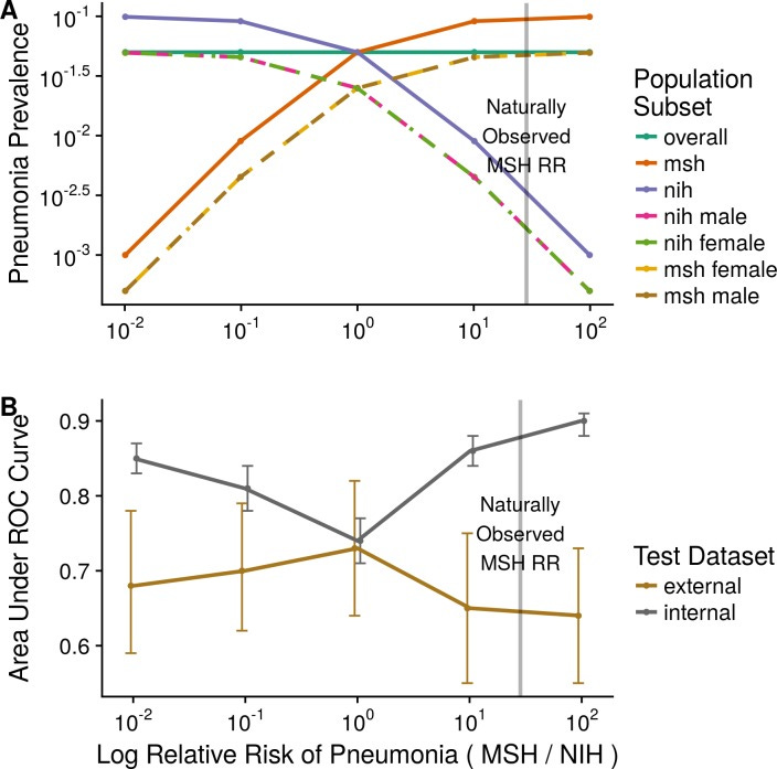
Fig. 2: Domain shift and model performance. This plot (adapted from Zech et al. 2018) illustrates how a model’s accuracy can drop when applied to a new context. The x-axis represents increasing difference in disease prevalence between two hospital domains (simulating a context shift), and the y-axis is model AUC (higher is better). Gray line: model’s performance on the internal (training-domain) test data; Brown line: performance on an external hospital’s data. As the prevalence gap grows (context more different), the model’s internal AUC stays high or even improves (overfitting to context), but the external AUC plummets[50][7]. In Zech’s study, extreme prevalence differences led to internal AUC ≈0.90 but external AUC barely ≈0.64[50][51]. Only when the prevalence was balanced (far left of plot) did the internal and external performance converge[52]. This experiment shows the model was exploiting context-specific clues (hospital identity correlated with prevalence) – a form of shortcut learning. The takeaway: models can appear highly accurate in their training context yet be brittle and unreliable when the context changes.[6][41]

Context dependence isn’t just about hospital or dataset; it can be biological context too. For example, a gene expression predictor of drug response might work in a controlled laboratory cell line panel, but fail in patient tumors, because the environmental context (cell culture vs human body) differs. Many early pharmacogenomic models had this issue – they didn’t translate well in vivo. Another example: a polygenic risk score for disease developed in one ethnic population often performs poorly in another population, because genetic architectures and environmental modifier factors differ – the context of genetic background shifts, and the model’s learned weights are slightly off-target.

In transcriptomics, context dependency is evident when comparing data across conditions: a gene signature for, say, inflammation derived from a specific tissue might not hold in another tissue or another species. We saw this in the human vs mouse tissue example where context (differences in when and how data were collected) confounded the comparison[27]. Even within a single-cell RNA-seq experiment, if you collect cells from different donors or labs, the “batch” effect blends with context – the donor’s genetics or lab protocols create context-specific gene expression baselines. Integration methods now attempt to separate what’s biologically shared vs what’s context-specific in such data.

A fine-grained illustration of context confounding comes from the same chest X-ray study: within a single hospital (Mount Sinai), the researchers found the CNN could perfectly distinguish portable chest X-rays (taken with a mobile machine, often for ICU patients) from standard departmental X-rays[53]. This is a context difference within one institution. Portable films had different image characteristics and were mostly from very ill patients. The CNN identified this context (100% accuracy distinguishing portable vs non-portable) and used it – indirectly predicting patient acuity rather than pneumonia per se. They later discovered this corresponded to different manufacturers of X-ray machines used in different hospital units[53]. This is an example of how hidden context (equipment differences) can leak into data. From the model’s viewpoint, it’s an easy way to cheat: ICU images likely mean sicker patients, hence higher pneumonia probability. The model doesn’t know it’s cheating; it just finds the correlation. But if we then tried to use that model on a general outpatient population (few portable X-rays), it might misfire completely.

The broader point is that AI models can be incredibly brittle when taken out of the context they were trained in. A quote from Recht et al. (2019) is pertinent: “current accuracy numbers are brittle and susceptible to even minute natural variations in the data distribution”[54]. In other words, even small shifts in context (a new batch, a slightly different patient population, a different scanner) can degrade performance. This is sobering for anyone hoping to deploy AI in clinical practice or trust AI findings in biology; one must validate models across varied contexts to ensure they’re learning the true signal, not context-specific quirks.

Open data example: The multiplicity of open datasets has both exposed this issue and offers a remedy. By trying their algorithms on datasets from different sources (which is possible when data are open), researchers can explicitly test generalization. For instance, there are multiple open chest X-ray datasets (NIH ChestXray14, CheXpert from Stanford, MIMIC-CXR from PhysioNet, etc.). A robust model for detecting, say, nodules, should work across all with minimal performance drop. If it doesn’t, that’s a red flag of context overfitting. Similarly, genomics has resources like GTEx (Genotype-Tissue Expression), an open dataset profiling gene expression across human tissues. A tissue-specific model can be tested on GTEx data from another tissue to see if it wrongly picks up tissue context. The availability of diverse datasets is a boon to stress-test AI models and identify when they rely on context.

To mitigate context issues, strategies include: collecting more diverse training data (so the model learns generalizable features), domain adaptation techniques (make the model’s features invariant to context differences), and meta-data inclusion (explicitly provide context as an input to the model, so it can adjust predictions accordingly, rather than inadvertently using context as a hidden proxy). But these are advanced solutions; the first step is always recognizing the potential for context to confound. The open research we cited demonstrates clearly that even expert-designed models can stumble on this — hence the emphasis in recent literature on external validation and reproducibility in different contexts.

Implications for Machine Learning Models in Biology

The challenges above are not just “data quirks” – they have profound implications for the reliability, interpretability, and reproducibility of machine learning models in biology. Here we summarize those implications and what they mean for both researchers and students:

Reproducibility and Reliability

Perhaps the greatest implication is on reproducibility. A model that performs brilliantly on one dataset but poorly on an independent dataset has limited scientific or clinical value. Unfortunately, as we have seen, issues like batch effects and context dependence often lead to such situations. Reproducibility crises in computational biology and medicine have been partly attributed to overfit models that do not generalize[22]. If a model’s result cannot be reproduced by others using different data or repeated experiments, trust in that model (and AI in general) erodes. This is why today there is heavy emphasis on independent test validation. For example, a genomics ML paper is expected to test its model on a completely separate cohort (often a publicly available dataset) beyond the one used for training; a lack of performance on that test indicates the model may have learned spurious patterns. The Nature survey and other analyses reinforce that without addressing data issues, irreproducibility will persist at a high rate[22][55]. Instructors teaching AI in biology must highlight this: a reproducible model is one that has learned biology, an irreproducible one likely learned the dataset.

One positive trend is the rise of consortia and challenges (e.g., DREAM challenges, Kaggle competitions on biomedical data) that provide training and hold-out test sets from different sources. Participants quickly learn that a top leaderboard score on the validation set means little if the final evaluation on an unseen set is poor. This is essentially forcing models to be robust to context and noise. Through such mechanisms, the community is getting better at developing models that are reliable. For instance, the DREAM Metastatic Cancer Challenge had teams train on one hospital’s pathology images and test on another’s – only those methods that handled stain differences and imaging protocol variations succeeded. These lessons have filtered into best practices published in papers and guidelines.

Risks in Data Interpretation and Scientific Discovery

When an AI model finds a pattern, scientists often try to interpret it to gain biological insight (e.g., “which genes are most important in this prediction?” or “what image features is the model attending to?”). But if the data were riddled with artifacts and the model latched onto them, any biological interpretation will be misleading or outright wrong. A model might highlight a gene not because it’s biologically central, but because that gene had a batch-specific bias. Or an imaging model’s heatmap might focus on the corner of an X-ray – perhaps because that’s where a hospital’s logo or a patient tag is located, not because of anatomy. If unaware, researchers might erroneously ascribe meaning (“the model paid attention to the lung apex; maybe the disease often starts there”), whereas in truth the model was reading a confounding text marker.

This is a significant risk: false biological knowledge. Earlier in the genomics era, many published gene signatures for diseases later turned out to reflect technical biases or batch differences. Those initial studies, using then-state-of-the-art statistical learning, reported lists of genes purportedly related to cancer prognosis, for example. Later, others showed that those gene lists could be proxies for lab effects or tumor sample site differences. As a result, very few early gene signatures replicated in later trials. This taught the field a cautionary tale: always check if your discovered pattern could arise from non-biological structure in the data.

In clinical AI, the stakes are even higher. If a model interprets an input in a confounded way, and we act on it, patients could be harmed. A trivial example: an AI model might predict that a patient has low risk for complication because in the training data those patients were from a hospital that tended to under-report complications (data bias). A doctor trusting that model could send someone home when in fact they are high risk. This underscores why interpretability and transparency in medical AI have been emphasized. Best practice requires documenting data provenance and ensuring the features influencing a model align with medical knowledge whenever possible[56][57]. When they don’t, that may signal a spurious correlation.

Moreover, the presence of noise and missing data can lead to overconfidence in results. Many standard ML algorithms will output a prediction and a confidence score. If the data distribution shifts (context change) but the model is unaware, it might still assign high confidence to its (now unreliable) predictions. This is dangerous in clinical settings (e.g., high-confidence incorrect diagnoses). It also misleads researchers – an overfit model can have very tight error bars in cross-validation, tricking one into thinking the result is solid, until an external test reveals a large error. Therefore, scientists now often use methods to assess model uncertainty and detect anomalies/out-of-distribution samples as part of their pipeline, especially in critical applications.

Model Brittleness and the Need for Robustness

We have repeatedly described models as “brittle” in the face of these data issues. Brittleness means the model’s performance or behavior changes drastically with slight perturbations in input or environment. This is antithetical to how we think of a good scientific model. We prefer models that gracefully handle variability – like how a well-designed diagnostic test works reliably across patient populations. When AI models break easily, it indicates they’re not truly capturing the underlying concept.

The research by Zech et al. on pneumonia detection is a prime example: the models were brittle to shifting hospitals[6]. Another instance of brittleness is seen in vision models that, when confronted with a bit of noise or a minor pixel shift, flip their predictions (this is related to adversarial examples, but even non-adversarial slight changes can affect an over-sensitized model). Biological data, being noisy, effectively tests models’ brittleness naturally. A robust model should be somewhat invariant to these small changes (like a slight change in a lab value shouldn’t completely alter a diagnosis). If an ML model trained on ideal data meets the wild variability of real data, it often fails fragilely.

There is an encouraging development: techniques like data augmentation (introducing noise and variability during training), regularization, and ensemble modeling can produce more robust models that don’t shatter at the first sign of distribution shift. For example, in histopathology image analysis, researchers found that augmenting training images with variations in color staining, blur, and rotation made models more resilient to images from other labs with different staining protocols[58][59]. The model learns to focus on pathology, not color intensity, if it has seen a spectrum of colors during training.

Ultimately, recognizing model brittleness has led to a mantra in the field: “Validate, then invalidate.” This means we not only validate models on independent data, but also actively try to make them fail by testing challenging scenarios (different batch, slightly corrupted data, etc.). By probing the breaking points, we understand where brittleness lies and can address it, either through retraining the model with more representative data or adjusting its architecture.

Ethical and Interpretative Cautions

An implicit but important implication is ethical: if certain biases (like missing data for certain subgroups) make models less accurate for those groups, that raises fairness issues. An AI tool might inadvertently perform worse for minority populations or under-served communities simply because the training data didn’t represent them well (a form of data representativeness problem). This has been observed in medical ML: e.g., a risk prediction algorithm trained mostly on data from one demographic may underpredict risk in another, contributing to healthcare disparities[3]. Ethically, we must be vigilant that “AI doesn’t make disparities worse,” to paraphrase Gianfrancesco et al.[2][3]. Ensuring data from diverse sources and understanding missingness patterns in socio-demographic context is part of responsible AI development.

From a scientific interpretative standpoint, all the above challenges urge a healthy skepticism in interpreting AI results. We should ask: “Is this real or a spurious correlation?” and trace findings back to raw data, checking for artifacts. Journals now encourage or require that ML papers share data and code so others can probe for issues. This open science approach helps catch problems (like the community did with the species gene expression case or with early COVID-19 X-ray models that were detecting context like portable machines or even the presence of a chest drainage tube rather than COVID per se).

Toward Robust and Reproducible AI: Best Practices and Conclusions

The reality that “biological data is messy” is not a cause for despair, but a call to action for better practices in AI-driven research. Awareness is the first step: as students and researchers, simply knowing about missing data, noise, batch effects, and context biases prepares you to critically evaluate data and models. As we’ve shown, a wealth of open-access studies have dissected these issues, and many provide guidelines on how to address them. Here we conclude with a summary of best practices (many adopted from the literature) to ensure AI models can truly thrive on biological data:

· Enrich and Clean the Data: Before jumping into modeling, perform rigorous data preprocessing. Impute missing values thoughtfully or use models that can handle missingness (and report how much data was missing)[8]. Remove or correct obvious errors and outliers (but keep track of what you remove). For example, one might exclude sequencing runs that failed QC or adjust measurements using calibration controls.

· Account for Batch and Laboratory Effects: Always ask how the data were generated. If there are known batches, include batch as a covariate in statistical models or apply batch correction algorithms before training the ML model[21][23]. Check batch balance across outcome classes (if imbalanced, your classifier might just learn batch). Use visualization (PCA, t-SNE plots colored by batch) to detect if batches cluster more than biological groups – a red flag requiring correction[27].

· Include Context Metadata When Possible: Rather than hoping a model ignores context, sometimes the best approach is to explicitly provide context as an input. For instance, in an EHR model, include hospital ID or patient demographics so that the model learns to factor those in (or use stratified models per subgroup). In genomics, if you have data from multiple studies, consider study ID as a random effect or one-hot feature. Paradoxically, telling the model about context can make it less likely to silently use context in a harmful way.

· Robust Training Techniques: Employ data augmentation and noise injection during training to make models more resilient. If you know measurements have ±5% noise, jitter your training data within that range. Use cross-validation schemes that respect batch (e.g., partition folds by batch or patient so you test generalization properly). Prefer simpler models when data is limited – complex models can overfit noise.

· Rigorous Independent Validation: Test your model on external data whenever feasible. This could mean temporal validation (data from a later time), geographic validation (another clinic’s data), or other public datasets. If performance drops, diagnose why (e.g., feature distribution shift, label differences) and address it. Public challenges and benchmarks are great for this – for example, submit your model to a DREAM challenge or use open leaderboards.

· Interpretation with Caution: Use explainable AI tools (like SHAP values for features, saliency maps for images) to inspect what the model is focusing on. Cross-check those against known biology or possible artifacts. If a handful of features or pixels drive the model, ask if they correlate with any technical factors. For image models, tools like TCAV (Testing with Concept Activation Vectors) can test if the model is sensitive to known confounders (e.g., does the model’s prediction score change if a hospital logo is present?). Such testing can uncover, for example, that a pathology AI was keying in on slide scanner identifiers.

· Reproducible Pipelines: Practice good data science hygiene – document every data processing step, use version control for code and environment, and when possible, share your data (or use available open data) so others can replicate and audit your findings. This makes it easier to spot if an issue (like batch effect) was inadvertently introduced or not handled. Reproducibility isn’t just about others trusting your work; it often helps you catch your own mistakes or assumptions.

· Stay Skeptical yet Curious: Finally, cultivate the mindset that any astonishing pattern might be “too good to be true”. Check the literature (as we did here) for similar cases and how they were resolved. On the flip side, be curious about new methods coming from the community: for example, data integration frameworks that explicitly model multiple sources to avoid batch effects[60], or causal inference techniques that try to learn cause-effect rather than just correlation (helpful in teasing apart true signal from confounding noise).

Biology is wonderfully complex, and data reflecting it will never be as tidy as we wish. But, as the field of AI in biology matures, we are developing the tools and knowledge to bridge the gap between AI’s assumptions and experimental reality. By emphasizing careful data handling and thorough validation, we can build models that are both powerful and trustworthy. The take-home message for students and practitioners is this: an AI model is only as good as the data we feed it. Understanding the nuances of that data — the missing bits, the noisy measurements, the batch quirks, the context behind it — is as important as understanding the algorithm itself. With open access datasets and literature shining light on these issues, we are better equipped than ever to make AI a true partner in biological discovery, rather than an unwitting generator of hype or bias.

In conclusion, the principle “AI assumes biological data is clean and representative, but real data is messy” should remain at the forefront of any bioinformatics or biomedical AI project. It’s a reminder to respect the data – to question it, clean it, and truly understand it – before and while leveraging AI. By doing so, we enable machine learning to reach its potential of yielding genuine biological insights and reliable clinical tools, built on a foundation of robust and reproducible science[20].

References

1. Flores, J.E., et al. (2023). Missing data in multi-omics integration: Recent advances through artificial intelligence. Front. Artif. Intell. 6:1162783. [1][14]

2. Yu, Y., et al. (2024). Assessing and mitigating batch effects in large-scale omics studies. Genome Biol. 25:21. [21][25]

3. Zech, J.R., et al. (2018). Variable generalization performance of a deep learning model to detect pneumonia in chest radiographs: a cross-sectional study. PLOS Med. 15(11): e1002683. [6][7]

4. Gianfrancesco, M.A., et al. (2018). Potential biases in machine learning algorithms using electronic health record data. JAMA Intern. Med. 178(11):1544-1547. [2][9]

5. Gilad, Y. & Mizrahi-Man, O. (2015). A reanalysis of mouse ENCODE comparative gene expression data. F1000Research 4:121. [27][29]

6. Lin, S., et al. (2014). Comparison of the transcriptional landscapes between human and mouse tissues. PNAS 111(48):17224-17229. [27]

7. Cardoso, F., et al. (2016). 70-gene signature as an aid to treatment decisions in early-stage breast cancer. N. Engl. J. Med. 375(8):717-729. [25]

8. Karimi, D., et al. (2020). Deep learning with noisy labels: Exploring techniques and remedies in medical image analysis. Med. Image Anal. 65:101759. [61][44]

9. Batch Effects Figure – adapted from Yu et al. (2024), Genome Biology 25:21. [62][36] (Creative Commons CC-BY-NC-ND 4.0 license)

10. Domain Shift Plot – adapted from Zech et al. (2018), PLOS Medicine 15(11):e1002683. [50][7] (Creative Commons CC-BY 4.0 license)

[1] [11] [12] [13] [14] [15] [16] Missing data in multi-omics integration: Recent advances through artificial intelligence - PMC

https://pmc.ncbi.nlm.nih.gov/articles/PMC9949722/

[2] [3] [4] [8] [9] [10] [17] [43] Potential Biases in Machine Learning Algorithms Using Electronic Health Record Data - PMC

https://pmc.ncbi.nlm.nih.gov/articles/PMC6347576/

[5] [18] [19] [20] [21] [22] [23] [24] [25] [26] [27] [28] [29] [30] [31] [32] [33] [34] [36] [37] [38] [39] [40] [55] [62] Assessing and mitigating batch effects in large-scale omics studies - PMC

https://pmc.ncbi.nlm.nih.gov/articles/PMC11447944/

[6] [7] [41] [46] [47] [48] [49] [50] [51] [52] [53] [54] [56] [57] Variable generalization performance of a deep learning model to detect pneumonia in chest radiographs: A cross-sectional study - PMC